Tom Thomson's "Sunset" 1915

Which comes first - the scene or the science?

My approach to studying a Tom Thomson skyscape is essentially a logical flow chart. All branches of science and nature can come into play eventually but I always start with the meteorology. The horizon is very low on the small panel making "Sunset" another skyscape and an observation of the weather for Tom Thomson. There are actual many "Sunset" works in Tom's portfolio. Lawren Harris and Dr. James  MacCallum were apparently running out of unique names for the growing number of Tom's skyscapes. 

The first question is what is the predominate cloud type? If the cloud is in the lowest levels of the atmosphere, one must apply the science of the planetary boundary layer (PBL). If the clouds are higher in the free atmosphere, then the Conveyor Belt Conceptual Model (CBCM) is the one you typically require. Conceptual models tend to point north by convention. They apply equally well when directed to the northeast or east should that be the direction of the system motion. 

"Sunset 1915" is a painting of clouds in the middle layers of the atmosphere. The diagnosis of Tom’s painting reduces to locating what part of the conveyor belt conceptual model (CBCM) was crossing his location while he painted. For your convenience, I have included important links that more thoroughly describe the features being discussed but if you have already followed these Blogs, you might be able to continue without that background information. Do not feel intimidated... it has taken me a lifetime to attempt to understand the weather that surrounds us everyday. Any challenges are the result of me not explaining it clearly enough... please forge onward. 

Tom Thomson, Sunset, 1915
Oil on composite wood-pulp board,
21.6 x 26.7 cm (8.5x10.5 inches)
  National Gallery of Canada, Ottawa

There are several give-away facts in Tom Thomson's "Sunset" from 1915. The backlit, sunset clouds clearly reveal the westerly direction that Tom was looking. If we had the date, we could narrow his view down to the nearest degree and the time to the minute. 

This is a warm conveyor belt and part of the larger conveyor belt conceptual model (CBCM) for mid latitude, large-scale synoptic storms. With the identification of this pattern, a wealth of information immediately becomes available to explain the current and future weather. The full explanation of the CBCM takes  a dozen blogs and those can be found starting with "Dancing with the Weather" as well as in several other locations. But there are still some very interesting things that can be discovered without diving too deep into the data. 

The significant expanse of altocumulus cloud reveals large scale dynamic lift in the atmosphere which is characteristic of the warm conveyor belt portion of the CBCM. This ascent occurs when air parcels ride the constant-energy (isentropic) surfaces for free. You might recall that these isentropic surfaces slope upward toward the north. You can actually see that slope in Tom’s painting!

The sharp edges to the multiple bands of clouds are the next important clue. These long and well-defined edges can only be deformation zones or the edges of gravity wave clouds. I may have been known as Mr. Deformation  because I found the answer to almost every question in a deformation zone. But not in this case! These are gravity waves and Tom included the clues in his painting. 

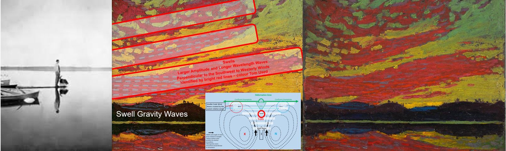
Tom's location within the Warm Conveyor Belt is the red circle
where both the wind gravity waves and swells are aligned in 
the same direction perpendicular to the wind within the
atmospheric frame of reference. There are some cloud clues
placing Tom in the left side of that circle as the wind waves 
are angled slightly across the swells - but I do not wish to
read too much into every brush stroke...

There are in fact two different types of gravity waves in Tom’s brush strokes – wind waves and swells. I blogged about these in "Wind Waves and Swells and Lines in the Sky" as well as a few other places. I am certain that Tom was within the red circle of the warm conveyor belt when he observed "Sunset". The accompanying slide from my "Tom Thomson Was A Weatherman" PowerPoint presentation will save some written words and includes that red circle for his location. 

The following graphic illustrates how smaller amplitude and shorter wavelength wind waves can be superimposed on the much larger amplitude and longer wavelength swells. Significant swells can be observed generated from strong winds long distances away - like the wake of a large boat being observed far away on the opposite shore of a lake. 

Both the wind waves and swells are aligned. This reveals Tom locations to be well south of the col in the deformation zone pattern where the atmospheric frame winds flow perpendicular to the swells generated by strong winds at the centre of the weather system. 

I added the lifted condensation level as the dashed red line in
this graphic to illustrate how it can dramatically change our
view of the cloudy wave crests and clear troughs of the
gravity waves as painted in "Sunset 1915"

Tom included the smaller amplitude wind waves - dashed grey lines.
Tom's grey lines correspond to the wind wave crests and thicker
amounts of cloud as they line up and extend beyond the edge
of the swell crests

In the accompanying graphic, I highlighted the larger amplitude swell crests within the red boxes. Note that the lifted condensation level must be below the equilibrium level in the wave pattern (above Option 4 and included as the dashed red line in the Wind Wave Plus Swell Graphic above). The relatively cloud free area in the swell trough is more narrow than the cloudy areas of the swell crest. If both crest and trough bands were the same width, the lifted condensation level would be found at the equilibrium level in the wave pattern. 

Tom was observing the atmospheric ocean. Those bands of clouds within the warm conveyor belt are large swells with the smaller wind waves superimposed. The clouds have sharp edges and occur at the same level in the atmosphere which is a characteristic difference from what one would expect and observe with deformation zones .. but that is another story. 

One final note.. the cloud on the right side of the panel and overhead are higher along the isentropic surfaces than the more distant clouds to the southwest. The orientation of the gravity wind waves actually turn clockwise with height. This veering of the wind direction with height reveals that warm air is being advected with those winds - something I blogged about in "Shifting Winds? Why?". This is consistent with the warm conveyor belt as well as it pumps warm and moist air northward, riding for free up the isentropic surfaces. 

From the preceding discussion, we can be very confident that Tom was within the red circled area of the CBCM. The deformation zone leading the high and thin cirrostratus was already far to the northeast. The wind waves were blowing in almost the same direction as the swell. The weather and possibly nimbostratus cloud were getting closer. 

Calm Waters, Sun Glint and the White Line

Now note the calm surface of the lake. The distant shore and the sky are mirrored perfectly in the calm waters.  The planetary boundary layer (PBL) has already decoupled from the increasing southwest to west flow aloft.  This could be the result of the quick development of the radiational inversion with sunset. An inversion occurs when the rapid cooling of the earth’s surface and adjacent air leaves the top of the planetary boundary layer relatively warm. Warm air overlying colder air is a stable configuration (inverted from the typical situation in the atmosphere) that prevents the wind in the free atmosphere from penetrating to the surface. The strong winds that created the gravity waves aloft could not get past the stable warm inversion and reach to the surface. 

The tranquil winds could also be the calm before the storm. I wrote about this process in a blog about the importance of the cold conveyor belt. Essentially the approach speed of the system might be nearly equal and opposite to the storm inflow winds along the cold conveyor belt. The two opposing wind components can balance out leaving the negligible surface winds as the calm before the storm. 

The other interesting feature of the water surface is the yellow line on the distant shore. This is sun glint from the calm water and results from the increasingly large water surface area subtended by the artist’s eye as you look at those reflective, glancing angles. Tom's vantage was very low - perhaps even from his canoe, so Tom painted the maximum amount of reflected line possible. A graphic from my presentation might help to explain this concept of sunset light reflected at glancing angles from distant water surfaces. 

The PowerPoint interaction of this slide is complicated with arrows
and interactions whizzing about. What it shows is that the viewer
sees more surface area at a glancing angle to the water. The larger 
viewing area reflecting more light to your eye explains the 
white or yellow line in this case that Thomson observed and painted.
Reflection greatly exceeds refraction at these glancing angle as well.
Refraction of light dominates reflection when the viewer looks
more directly down into the water.  

Finally, the rich red colours in the clouds and orange shades in the sky were strongly influenced by the May 22nd, 1915 eruption of Lassen Peak in north central California. The Lassen Peak eruption was tiny compared to the major eruption of Mount St. Helens in 1980 but the effects on the sky were still noticed by the artists in Algonquin - and after all, they painted what they saw. 

Sulphur dioxide spewed from volcanoes reacts in the atmosphere
to form sulphate aerosols (aerosols are tiny, suspended particles in the air).
Rayleigh scattering by volcanic ash and aerosols preferentially scatter the
shorter blue wavelengths out of the sun's direct beam. The direct beam passes
through a long path of atmosphere at sunrise and sunset leaving only
longer wavelengths of orange and red to illuminate the scene.

My PowerPoint slide shows Rayleigh scattering of short wavelength light
out of the direct beam from the sun. The sulphate aerosols from
volcanoes do a good job at removing the longer green wavelengths
as well. Mie scattering forward scatters the light that the clouds intercept
… which is red and longer wavelengths only. Tom saw red clouds. 

A "simple" sunset painting probably completed in 30 minutes or less is far from being straightforward. I spent a lot longer than that just trying to explain what Tom observed. Tom certainly worked on this small 8.5 by 10.5 inch panel using his sketch box. One can see the paint smears where he slid the panel into the carrying portion of that box upon completion. Overcast nimbostratus skies were not that far to the southwest when he tucked this panel into the paint box. The elevated portions of some brush strokes were even flattened when he later stacked this work with others before the oils were fully cured. Tom characteristically did not even bother to sign this little gem - the TT 1917 estate stamp can be faintly seen in the lower right. 

The lesson from a close examination of  Thomson's art is that if you paint nature as you see it, you will also be recording the truth. Tom certainly painted what he saw. He did not make any of this science up. Tom might not even have fully understood what the clouds were really saying but he was listening ..

Weather is always exciting. Every cloud and every line have stories to tell if we only learn the vocabulary. Do not be too concerned about remembering all of this science. None of this is going to be on any exam. My goal is simply to reveal how much science can be discovered within the brushwork of Tom Thomson so that we can all appreciate his real motivation and genius.  

As an aside, this painting is dated 1915 but the shoreline bears an acceptable correspondence to hills looking southwest into Carcajou Bay from where Tom Thomson may have sketched the Jack Pine - a short stroll south of the Out-Side-In. Thomson painted around Grand Lake in 1916  when he was working out of Achray as a fire ranger.  Tom wrote to Dr. MacCallum "Have done very little sketching this summer as the two jobs don't fit in." 

Another potential solution is that the date for the painting is accurate and the painting location was Tom's favourite campsite on Hayhurst Point. Tom would have been looking southwesterly toward the sunset possibly on the evening of Sunday, May 23rd, 1915. The sulphate aerosols from the volcanic eruption would have been just arriving at Canoe Lake. See "Tom Thomson's Sunset Sky, Spring 1915" for more explanation about the timing of this painting. 

Earning a salary can get in the way of making art. I was fortunate to find two loves in meteorology and art. Weather pays the bills and art feeds the soul. 

Thank you again to my friend Professor Edward Lozowski for his guidance in constructing this post.

Warmest regards and keep your paddle in the water,

Phil the Forecaster Chadwick

PS: Give yourself a Gold Star if you finished reading the post and got this far while following most of the science. The science gets easier with repetition. Meteorology is not rocket science - it can actually be more complicated. 

PSS: For the Blog Version of my Tom Thomson catalogue raisonné, Google Search Naturally Curious "Tom Thomson Was A Weatherman - Summary As of Now" or follow this link “http://philtheforecaster.blogspot.com/2022/10/tom-thomson-was-weatherman-summary-as.html”