Tom Thomson's Autumn Clouds Fall 1915

There is an element of a detective story in the Creative Scene Investigation (CSI) of each of Thomson's weather observations. The Who, What, When, Where and Why of the story always starts with just the image. That is all we have. The cloud types and wind that Tom painted can only be found in one portion of a weather system. Please let me explain. The story started decades aog...

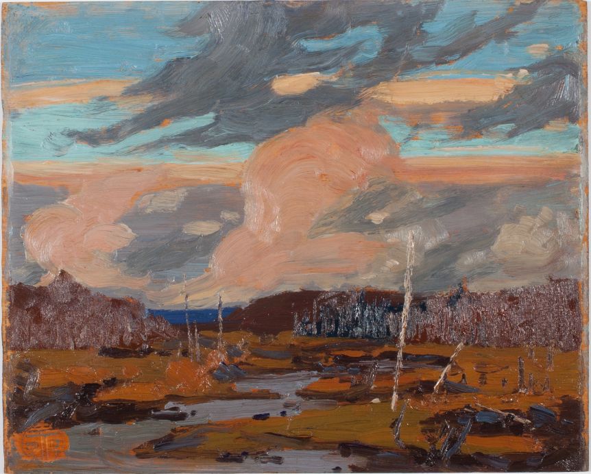Autumn Clouds Fall 1915
Oil on wood panel 8 9/16 x 10 9/16 in. (21.8 x 26.9 cm) 
Tom's Paint Box Size, 1915.75  

I was very fortunate to attend a lecture by Roger Weldon in 1981 while working at the Alberta Weather Centre in Edmonton. Weldon's work on storm patterns and specifically deformation zones was illuminating! His words opened a whole new world of scientific inquiry. 

It took a couple of years of fermentation and working with the new satellite data "for the penny to drop". The Eureka moment came on a 1983 night shift at the Atlantic Weather Centre in Bedford Nova Scotia. Every line in the atmosphere was a deformation zone when viewed from the atmospheric frame of reference - something that the new satellite data allowed. Everything made immediate sense when examined while moving with the atmosphere. The earth (a spinning ball with a thin and fragile skin of atmosphere) was not even close to being the perfect frame of reference. "Humans" were not the centre of the universe. 

The current conceptual model of the deformation zone (above) took years of further investigation. Some consistent terminology needed to be invented to differentiate between paired and companion vortices that differentiated between the swirls. Swirls that were across the deformation zone from each other were "paired" and responded in opposite directions to changes in confluent asymptote curvature. The "companion" swirls straddled the inflows to the col along the axis of contraction. They were simply cross-sections through the "3-D smoke ring" generated by the system relative wind. These swirls reacted to the inflow wind speed and deformation zone curvature. The shape of the two divergent confluent asymptotes that comprise the axis of dilatation (deformation zone) also contained information on system motion, thermal advections and stability. Deformation zones are independent of time and space scales and can be stacked vertically to diagnose changing stability due to advections. The deformation zone became my new bestie!

For further background information, consider "A Closer Look at Lines in the Sky" and "The Swirls and Deformation Zone Revisited" among the many times I have written on the subject. Most people are challenged by a frame of reference other than their own experience. I visited that material in "Down to Earth Meteorology" and "A Jet Streak with a Paddle" as well as several other posts. My strategy was to attempt different approaches to the same material until one reached the client. We all see things through different filters and lenses. 

The concept that a cold front was actually a deformation zone received a luke-cold reception (actually frosty) when I got to the Atmospheric Environment Service (AES) Training Branch. I probably did not explain the ideas succinctly (I still stuttered especially when I got nervous).  A warm front is also a deformation zone along with every other edge of moisture you care to scrutinize.  Examining atmospheric processes from the vantage of a moving perspective was not easy in 1985. A representative from the Ontario Weather Centre (OWC) was sent to learn my approaches to satellite imagery but spent the time in the cafeteria. I persisted but it took decades and the effort continues today within these blogs. New computer approaches to data display are making the atmosphere come alive even on your phone.

Tom's "Autumn Clouds" had to be along a cold front. The wind shift that Tom recorded also places him in a very specific location along that deformation zone. The following graphic will explain that better than words. 

The following graphic describes the diagnosis of the cloud types and winds painted by Tom.

The cumulus clouds were triggered by the cold frontal passage. The individual cells leaned forward toward Tom with the strong southerly to southwesterly winds aloft. The surface winds were reduced by friction in the planetary boundary layer (PBL) while those aloft were largely unaffected by the rough terrain and were thus stronger.

The turbulent stratocumulus clouds were paralleling the cyclonic companion winds of the dry conveyor belt. The instability along the cold front provided the necessary conditions for those Langmuir streaks. 

Both the cumulus and stratocumulus clouds locate Tom at the cold front of the weather system but there is more to be discovered in the mid-levels of the atmosphere...

The conveyor belt conceptual model that I tend to use in these blogs is for a mature weather system. Heat and moisture must follow constant energy surfaces on their journey from the source region in the tropics to the poles. Three adiabatic levels are good summaries of this flow. The highest flow (yellow in the graphic below) symbolizes the cirrus level. The orange flow is for mid-level moisture (altostratus and altocumulus) and the red level is reserved for low-level moisture. 

This is a big part of the energy balance of the planet moving heat, moisture and momentum (as well as electricity) around the globe. The high-level cirrus layers are typically confined to the warm side of the jet stream. As the low (vortex) intensifies and the system slows down, the original vortex occludes. This means that the surface wave and fronts (and cirrus) keep moving with the jet stream. The surface wave remains attached to the vortex only by an occlusion or a trowal. The "trowal" is a Canadian invention meaning a "trough of warm air aloft" since the characteristics of the elevated air mass (the occluded front) are often not distinguishable at the surface. 

Tom was painting a weather system that was in the early stage of occlusion. The mid-level cloud following the mid-level adiabatic surface (orange layer in the accompanying graphic) was wrapping westward to the occluding low-pressure area (cold low or vortex). The satellite image on the right side of the graphic shows a fully occluded weather system with bands of moisture wrapping around a cold low. This is a frequent occurrence in the atmosphere including January 13th, 2024 as I write this post (satellite image below).

Often, satellite imagery provides the first clue that a weather system is occluding. The cyclone (vortex) in the upstream cold trough starts to really wind up. The strengthening circulation that occurs at the mid and lower levels in the atmosphere draws the mid-level moisture around the cyclone and out from under the cirrus cloud shield. This mid-level "hang-back" moisture may be upstream from the warm conveyor belt but is still an important part of the storm. This moisture is also frequently referred to as the comma head of the storm. The track of the occluding low is a good place to start when forecasting the swath of heavy precipitation. This is what Thomson saw and painted. Tom observed the layer of altostratus reaching back to the low. 

The following graphic is a close-up of the viewing angles for the leaning cumulus at the surface cold front and the turbulent stratocumulus streaks along the frontal surface. The mid-level altostratus is also depicted forming in the overrunning above the warm frontal surface and being drawn westward along the occlusion and around the vortex. 

Mid-level moisture is witnessed as it climbs the warm frontal surface and is drawn around the intensifying vortex at the red X. Satellite water vapour imagery often displays several layers of cloud at different levels of the atmosphere swirling around the vortex. The above sketch suggests that the altostratus had not yet completed one swirl around the vortex. More vigorous or older vortices can cause that moisture to make several trips around the low. This graphic illustrates the simplest case occlusion. 

These occluding systems gradually move slower as they intensify and typically become a nearly stationary and vertical cutoff cold low while the warm moist air of the warm conveyor belt continues to move away with the jet stream. This is the occlusion process described in just a few words. The cold low will remain stationary producing lots of weather, wind and precipitation until another impulse of atmospheric energy (an atmospheric wave rippling along the jet stream)  approaches to eject it back into the flow. When the upstream pulse of energy gets within "twenty degrees of latitude", the cold low moves back into the jet stream flow. 

The following graphic assembles all of the puzzle pieces into a solution. The occlusion process was just starting and not developed sufficiently to block the setting sun.

This is all old-school meteorology before the rapid advances of numerical weather prediction (NWP). This approach dates from when understanding the atmosphere was an observational science of the real atmosphere through satellite and radar and not the tweaking of NWP simulations and equations.

The clues analyzed within the painting require that Tom was looking northwestly to observe these cloud types which were still illuminated by the late afternoon sun. The surface cold front was crossing his easel while the hang-back altostratus was being drawn westward around the occluding cold low. 

At this point, I reached out to my Thomson friends inquiring if they might know where "Autumn Clouds Fall 1915" was completed. The result came back in minutes… and it was a match.

Tom accurately observed and painted the weather so that a century later, one can deduce where he was and what he saw. We already knew who! The late afternoon colours of the clouds even reveal when. The colours of the terrain and vegetation suggest that the timing of this plein air painting was also quite late in autumn before the snow started to fall. We can even guess why. The weather and wind were unusual and just had to be recorded in oils - an occluding cold low was just to the west.

Discovering this story allows us to almost be there beside Thomson while he painted, experiencing the weather with him. The art can become an experience beyond the simple pleasure of enjoying the brush strokes and pigments. Sharing this with others is a big motivation for these posts. The opportunity to do so would be lost without the knowledge and generous support of my Thomson friends.

Inscription recto: 

• l.l., estate stamp 

Inscription verso: 

• c., estate stamp; 
• c., in red crayon, Laidlaw; 
• u.l., in graphite, 17 (underlined); 
• u.l., in red crayon, L; 
• u.l., in graphite, WCL (circled); 
• u.r., in graphite, Not to be touched / up round stamping / J.MacD. (underlined); 
• u.r. quadrant, in red pencil, 29 (circled); 
• c.r., in red ink, Gift to McMichael, R.A. Laidlaw (underlined); 
• u.r. quadrant, in graphite, No. / 51 Mrs. Harkness; 
• c.l., in green ink, 12 McMichael Canadian Art Collection, Kleinburg (1966.15.25) 

Provenance:

• Estate of the artist;
• Elizabeth Thomson Harkness, Annan and Owen Sound 
• R.A. Laidlaw, Toronto
• McMichael Canadian Art Collection, Kleinburg (1966.15.25). Gift of R.A. Laidlaw, Toronto, 1965

This is another one of those panels from the stack of Thomson's paintings retrieved from the Shack. In the spring of 1918 Lawren Harris and J.E.H. MacDonald had a virtually impossible task to sort through Tom's efforts of the previous three years. Sadly large chunks of paint flaked off the panel where the estate stamp was applied. 

This painting went to Thomson’s eldest sister upon his passing. Elizabeth's husband was Thomas “Tom” J. Harkness who was appointed by the Thomson family to look after the affairs of Tom’s estate. T. J. and Elizabeth lived in Annan, Ontario, just east of Owen Sound. From Elizabeth, aka "Mrs. Harkness", the painting went to Robert .A. Laidlaw and then to the McMichael in 1965.   

Warmest regards and keep your paddle in the water,

Phil Chadwick

PS: Tom Thomson Was A Weatherman - Summary As of Now contains all of the entries to date. 

PSS: Should you wish to have Creative Scene Investigation applied to one of Thomson's works that I have not yet included in this Blog, please let me know. It may already be completed but needs to be posted. In any event, I will move your request to the top of the list. If you made it this far, thanks for reading! There is a lot of science in this small panel and I wanted to cover most of it...

PSSS: It has taken time and effort since the Training Branch in 1985 but the unifying theories of lines and swirls observed from an atmospheric frame of reference have gained wide acceptance elsewhere through the support of COMET, NOMEK and EUMETSAT. I met some wonderful friends on those trips. These posts hopefully will spread the ideas to everyone so that like Tom Thomson, they might appreciate the beauty of the weather and the science that explains it. The conceptual models and meteorology are also blogged in "The Art and Science of Phil the Forecaster".